
Once upon a time I wrote a post about building a toy TF-IDF keyword search engine. It has been one of the more popular posts I’ve written, and in this age of AI I felt a sequel has been long overdue.
It’s pretty fast (even though it’s written in pure Python), it ranks results with TF-IDF, and it can rank 6.4 million Wikipedia articles for a given query in milliseconds. But it has absolutely no context of what words mean.
>>> index.search('alcoholic beverage disaster in England')
search took 0.12 milliseconds
[]
Not a single result, even though the London Beer Flood is sitting right there. For context, the London Beer Flood is an accident that occurred at a London brewery in 1814 where a giant vat of beer burst and flooded the surrounding streets. That’s very much an “alcoholic beverage disaster in England”, but our keyword search engine doesn’t know that “beer” and “alcoholic beverage” are similar concepts, or that “London” is in “England,” or that a “flood” is a type of “disaster.” It only knows how to match strings 1.
In the original post, we built an inverted index with TF-IDF ranking, and recently the project underwent some modernization with Hugging Face datasets and proper tooling. The core search engine hasn’t changed: tokenize, stem, look up matching documents, rank by term frequency weighted by inverse document frequency. It works great when your query uses the same words as the documents. But when you don’t know the right words to search for, you end up with empty results and sad emojis.
By the end of this post, we’ll have a vector-based search mode that captures meaning, in around 200 lines or so of Python 2:
>>> vector_index.search('alcoholic beverage disaster in England', k=3)
[('1900 English beer poisoning', 0.6237),
 ('United States Industrial Alcohol Company', 0.5980),
 ('Timeline of British breweries', 0.5732)]
All the code is on GitHub.
What are embeddings?
The TF-IDF search engine already represents documents as vectors, in a way. Each document becomes a sparse vector with one dimension for every unique word (or token really) in the corpus. If the corpus has 500,000 unique words, each document can be represented as a vector with 500,000 dimensions, most of which are zeroes. One way to think about this is that every unique word has an index on an array of length 500,000 (say beer is index 42). Then every document that has the word beer in it, would have a 1 (or the number of times the word beer occurs in the document, i.e. term frequency) on index 42 (and zeroes for all the words that aren’t in the document). The problem is that “beer” and “alcoholic beverage” end up on completely random positions/dimensions with no relationship encoded between them.
Embeddings take a different approach. Instead of one dimension per word, a neural network learns to compress text into a dense vector of a few hundred dimensions, where every value is meaningful.
The main idea is that if you just look at enough data, you’ll observe similar things having similar words co-occur more often. The model is trained on billions of sentences, and it learns that similar meanings should end up near each other in this vector space. “King” and “queen” are close together. “King” and “bicycle” are far apart. “Beer” and “alcoholic beverage” are neighbors3.
The key insight is that these vectors capture semantic relationships, not just lexical ones. The model has never seen our specific query or our specific documents, but it has learned enough about language to know that a query about “alcoholic beverage disaster in England” should be close to a document about a beer flood in London.
If you want to go deep on how these models work beyond this very high level gist, I highly recommend Jay Alammar’s Illustrated Word2Vec blog post for the foundational intuition, and the Sentence-BERT paper for the specific architecture we’ll use. You don’t need to understand the internals to use them, just like you don’t need to understand combustion engines to drive a car.
Generating embeddings
We’ll use the sentence-transformers library for this; essentially there’s a whole bunch of open models available on the internet, trained on different datasets and languages, output different dimensions, use different model architectures, etc. We’re not going too worry too much about that and just load a pre-trained model and call encode:
from sentence_transformers import SentenceTransformer

# the first time you do this it'll download the model weights
model = SentenceTransformer('all-MiniLM-L6-v2')
vector = model.encode('alcoholic beverage disaster in England')
# vector is a numpy array of 384 floats
len(vector)  # => 384
# array([ 4.01491821e-02, -1.56203713e-02,  3.25193480e-02, -4.24171740e-04,
#         7.81598538e-02,  4.59311642e-02, -1.13611883e-02,  1.07017970e-02
# ...
#         8.66697952e-02, -7.92134833e-03,  4.44980636e-02, -1.87412277e-02],
#      dtype=float32)
That’s it. The model takes a string and returns a 384-dimensional vector that captures its meaning. The all-MiniLM-L6-v2 model is small (80MB), fast, and surprisingly good for general-purpose semantic search4.
If you prefer a hosted API, OpenAI offers an embeddings endpoint:
from openai import OpenAI

client = OpenAI()
# or if you prefer OpenRouter
# client = OpenAI(base_url=https://openrouter.ai/api/v1, api_key="sk-or-v1-...")
response = client.embeddings.create(
    input='alcoholic beverage disaster in England',
    model='text-embedding-3-small'
)
vector = response.data[0].embedding
len(vector)  # => 1536
# [0.0035473527386784554,
# 0.030878795310854912,
# 0.03244471549987793,
# 0.03686774522066116,
# -0.02967001684010029,
# -0.018530024215579033,
# 0.027856849133968353,
# 0.010542471893131733,
# -0.03247218579053879,
# -0.0033705001696944237,
# ...
# N.B.: note that this is a list of floats, not a NumPy array!
N.B.: pro-tip, OpenRouter.ai has tons of models available and has an OpenAI-compatible API if you want to compare different models. Many of the models they offer even have free tiers, although at time of writing there seem to be no free embedding models.
The tradeoffs are straightforward: sentence-transformers is free because it runs locally, and produces 384-dimensional vectors. OpenAI costs money, requires a network call, and produces 1536-dimensional vectors. For this project, free and local wins (free is my favorite price), and the smaller vectors will be easier on our memory budget later.
It also comes with batch encoding, which we’re going to need when we’re embedding 6.4 million documents:
vectors = model.encode(
    [doc.fulltext for doc in documents],
    batch_size=256,
    show_progress_bar=True
)
This will embed our documents in batches of 256, showing a pretty progress bar so you know roughly how long your coffee break should be5.
We’re going to process our 6.4 million documents in chunks rather than loading everything into memory at once. The implementation on GitHub processes documents in groups of 10,000, saving intermediate embeddings as checkpoints. I got sick of having to start over while I was writing this because something crashed halfway through.
If you’d rather skip the multi-hour encoding step, I’ve uploaded the pre-computed embeddings to Hugging Face 🤗 so you can download them and start searching right away. Just move the JSON and .npy files into data/checkpoints and run uv run python run_semantic.py.
The memory problem
Let’s do some napkin math (it’s the best math). We have 6.4 million documents, each represented by a 384-dimensional vector of 32-bit floats:
$$6{,}400{,}000 \times 384 \times 4 \text{ bytes} \approx 9.2 \text{ GB}$$
That’s not an insignificant amount of RAM, and that stuff comes at a premium these days.
One easy win we can have here: we’ll store the vectors as 16 bit floats instead of 32 bit. The precision loss is negligible for ranking because we’re just comparing relative similarity scores, not doing stuff that’s sensitive to rounding errors like launching rockets:
$$6{,}400{,}000 \times 384 \times 2 \text{ bytes} \approx 4.6 \text{ GB}$$
Better, but still a lot. Add the documents themselves and you’re past what a typical laptop has to spare. My MacBook would start sweating just thinking about it.
The solution is numpy.memmap. Instead of loading the entire matrix into RAM, we memory-map the file: the operating system maps it into our address space but only loads pages from disk as we access them, and evicts them when memory gets tight. We get the programming model of “everything in RAM” without actually needing all that RAM. Also maybe don’t do this in production systems.
import numpy as np

# create a memory-mapped file to write embeddings into as we go
matrix = np.lib.format.open_memmap(
    "vectors.npy", mode="w+", dtype=np.float16,
    shape=(num_documents, 384),
)

# write chunks of embeddings directly to disk
for i in range(0, num_documents, chunk_size):
    chunk_vectors = embed_batch(model, chunk_texts)
    matrix[i:i+len(chunk_vectors)] = chunk_vectors.astype(np.float16)
matrix.flush()

# later, load it back memory-mapped for search
matrix = np.load("vectors.npy", mmap_mode='r')
# matrix looks, acts and quacks like a normal numpy array
# lives on disk, the OS pages in what we need
This works because the OS virtual memory system is really good at this. It maps the file into the process’s address space, loads 4KB pages on demand when you touch them, and transparently evicts pages under memory pressure. For our search workload, where each query touches every row but only briefly, the OS can page data in and out efficiently. We don’t need to write any caching logic ourselves.
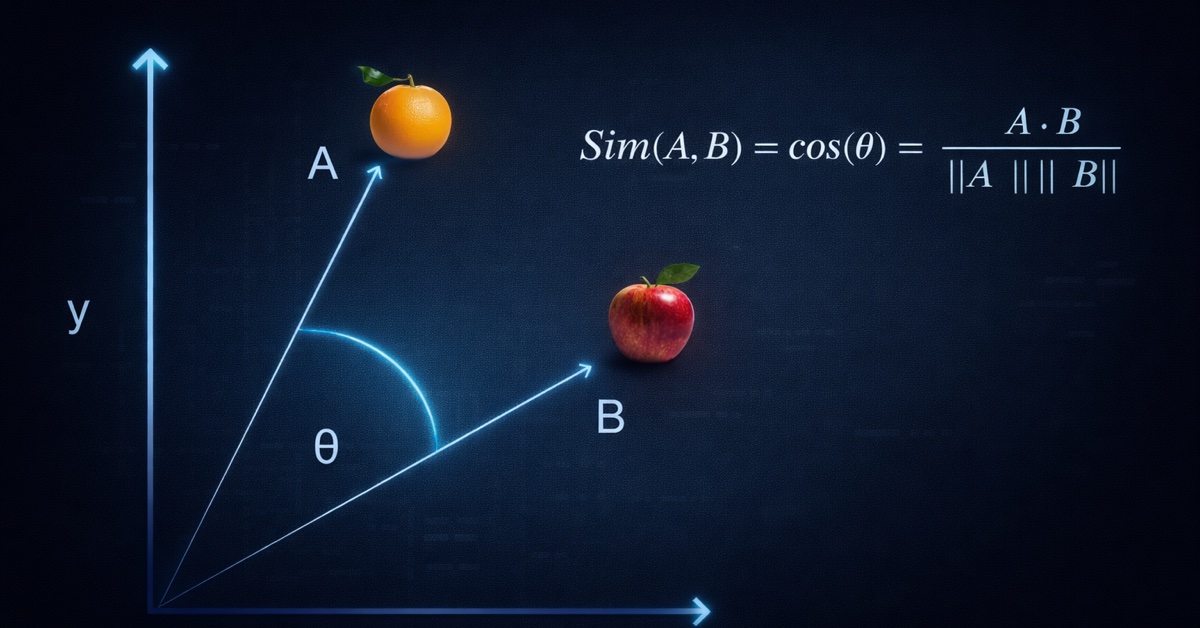
Cosine similarity
Now we have vectors for our query and for every document. How do we find the most similar ones? We need a way to measure how “close” two vectors are in our 384-dimensional space. The standard measure for this is cosine similarity.
The formula
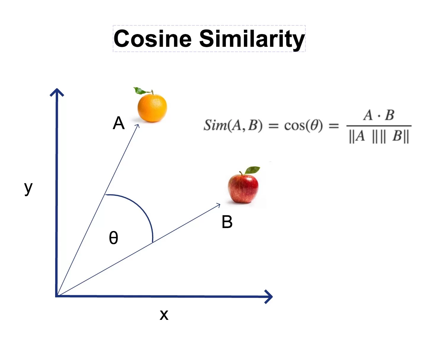
Cosine similarity measures the cosine of the angle between two vectors. Two vectors pointing in the same direction have a cosine of 1. Two perpendicular vectors have a cosine of 0. Two vectors pointing in opposite directions have a cosine of -1.
$$\cos(\theta) = \frac{\mathbf{A} \cdot \mathbf{B}}{|\mathbf{A}| |\mathbf{B}|}= \frac{\sum_{i=1}^{n} A_i B_i}{\sqrt{\sum_{i=1}^{n} A_i^2} \times \sqrt{\sum_{i=1}^{n} B_i^2}}$$
Don’t let the formula intimidate you. It has three parts:
- Numerator (the dot product): multiply each pair of corresponding elements and add them up. If two vectors have large values in the same dimensions, this number will be big.
- Denominator (the magnitudes): compute the “length” of each vector and multiply them together. This normalizes the result so it doesn’t depend on how long the vectors are, only their direction.
- Result: a number between -1 and 1, where 1 means identical direction, 0 means unrelated, and -1 means opposite 6.
A naive implementation
Let’s build it from scratch in plain Python, because I think seeing the pieces helps:
import math

def dot_product(a, b):
    return sum(ai * bi for ai, bi in zip(a, b))

def magnitude(v):
    return math.sqrt(sum(vi ** 2 for vi in v))

def cosine_similarity(a, b):
    return dot_product(a, b) / (magnitude(a) * magnitude(b))
And it does what we’d expect:
>>> cosine_similarity([1, 2, 3], [1, 2, 3])
1.0
>>> cosine_similarity([1, 2, 3], [-1, -2, -3])
-1.0
>>> cosine_similarity([1, 0, 0], [0, 1, 0])
0.0
Identical vectors, opposite vectors, and perpendicular vectors. The math checks out.
The problem at scale
Here’s the thing: we need to compute cosine similarity between our query vector and every single document vector. That’s 6.4 million similarity computations, each involving 384 multiplications and additions. That’s about 2.5 billion floating-point operations per query. That naive Python implementation would take… a while.
The normalization trick
There’s a pretty elegant optimization trick we can do though. If we normalize all vectors to unit length (magnitude = 1) at index time, the denominator of the cosine similarity formula becomes $1 \times 1 = 1$. The entire formula can be simplified to just the dot product:
$$\cos(\theta) = \mathbf{A} \cdot \mathbf{B} \quad \text{(when both vectors have unit length)}$$
And a dot product between a matrix and a vector? That’s exactly what NumPy was made for. It drops into optimized BLAS routines7 that use SIMD instructions, cache-friendly memory access patterns, and all the other tricks that make NumPy fast:
import numpy as np

# normalize all document vectors once at index time
norms = np.linalg.norm(matrix, axis=1, keepdims=True)
matrix /= norms

# at search time, normalize the query and dot product
query = query_vector / np.linalg.norm(query_vector)
scores = matrix @ query  # cosine similarity with ALL 6.4M documents
That matrix @ query line computes cosine similarity against every document in one shot. NumPy upcasts the float16 matrix to float32 on the fly during the multiplication, so we get full precision where it matters (the computation) while keeping the storage compact. On my laptop, this takes about 2 seconds for 6.4 million documents. Not bad for a brute-force search on a MacBook.
The VectorIndex class
Here’s the full class that ties everything together:
class VectorIndex:
    def __init__(self, dimensions=384):
        self.dimensions = dimensions
        self.documents = {}
        self._matrix = None

    def build(self, documents, vectors):
        for i, doc in enumerate(documents):
            self.documents[i] = doc

        self._matrix = np.array(vectors, dtype=np.float32)
        # normalize to unit vectors so dot product = cosine similarity
        norms = np.linalg.norm(self._matrix, axis=1, keepdims=True)
        norms[norms == 0] = 1  # avoid division by zero
        self._matrix /= norms

    def search(self, query_vector, k=10):
        # keep the query in float32, numpy will upcast the
        # matrix (which may be float16) automatically during matmul
        query = np.array(query_vector, dtype=np.float32)
        query = query / np.linalg.norm(query)
        scores = self._matrix @ query

        # find top-k results without sorting the entire array
        k = min(k, len(self.documents))
        top_k = np.argpartition(scores, -k)[-k:]
        top_k = top_k[np.argsort(scores[top_k])[::-1]]

        return [(self.documents[int(i)], float(scores[i])) for i in top_k]
Most of this should look familiar from the explanation above, but there’s one trick worth calling out: np.argpartition. When you only want the top 10 results out of 6.4 million, sorting the entire array is wasteful. argpartition runs in $O(n)$ time and gives us the indices of the top-k elements (unordered), and then we only sort those k elements. It’s the difference between sorting a phone book and just pulling out the top 10 entries 8.
Keyword vs. semantic: where each wins
Now that we have both search modes, let’s see how they compare:
| Query | Keyword search | Semantic search |
|---|---|---|
| “London Beer Flood” | Exact match, instant | Also finds it (0.74) |
| “alcoholic beverage disaster in England” | Nothing | 1900 English beer poisoning, Timeline of British breweries |
| “python programming language” | Lots of results | Python syntax and semantics, CPython, Python compiler |
| “large constricting reptiles” | Nothing | Outline of reptiles, Giant lizard, Squamata |
| “color” vs “colour” | Only matches exact spelling9 | Understands they mean the same thing |
The pattern is clear. Keyword search is precise – when your query matches the words used in the documents, it’s fast and reliable. Semantic search understands meaning – it bridges the vocabulary gap between how you phrase your query and how the document was written. “Alcoholic beverage disaster” finds beer poisoning articles. “Large constricting reptiles” finds squamates. Neither query shares a single word with the documents it found.
They’re not competing approaches. They’re complementary. So what’s next?
What’s next: hybrid search
We now have two search engines: one that matches keywords, and one that understands meaning. What if we combined them? Use keyword search for precision on exact terms, semantic search for understanding meaning, and blend the scores together.
That’s actually what modern search engine implementations like Elasticsearch, Vespa, and Pinecone do under the hood. It’s called hybrid search, and it’s what we’ll build in part 3. Stay tuned.
We applied some standard tricks to increase the likelihood of strings matching, but that only gets us so far, at the cost of reducing precision. ↩︎
Tbf it’s 200 lines that plumb a bunch libraries together, I’m not reimplementing the
transformerslibrary here 😅 The goal is to have an illustrative example of how this technology can be applied in a search engine context. ↩︎The original insight dates back to Word2Vec (2013), where researchers at Google showed you could learn word vectors by predicting surrounding words. The famous example:
vector("king") - vector("man") + vector("woman") ≈ vector("queen"). Modern sentence-transformers build on this idea but operate on entire sentences rather than individual words. ↩︎The
all-MiniLM-L6-v2model is a good balance of speed and quality. I’m also on an M4 MacBook so there’s only so much I can ask of the processor to embed 6.4m documents in a reasonable amount of time. There’s tons of models out there, with various different specializations (trained on multiple languages likebge-m3or much higher dimensionality to capture wider ranges of meaning better like theQwen3family of embedding models). The MTEB leaderboard ranks models by various benchmarks, so which one to pick depends on your use case and how many GPUs you can afford. ↩︎On a CPU, encoding 6.4 million documents takes a few hours. On a GPU, it could be more like 20 minutes. If you have a CUDA-capable GPU,
sentence-transformerswill use it automatically. I’m on Apple Silicon, and it’ll use thempsbackend leveraging the Apple GPU, but while faster than CPU it’s still significantly slower than an Nvidia GPU. ↩︎In practice,
sentence-transformerembeddings rarely produce negative cosine similarities. The values tend to cluster between 0 and 1, with most unrelated pairs landing around 0.1-0.3. Don’t expect to see many -1.0 values in the wild. ↩︎BLAS (or Basic Linear Algebra Subprograms) and LAPACK (Linear Algebra Package) are linear algebra libraries, often written in Fortran, that have highly optimized low-level routines for doing linear algebra. These libraries have been around for ages, and are what makes NumPy so fast. It’s like calling upon the Wisdom of the Ancients™ ↩︎
Technically,
np.argpartitionuses the introselect algorithm, which is a hybrid of quickselect and median-of-medians. It guarantees $O(n)$ worst-case, which is nice. ↩︎Our keyword search does have stemming, so it would catch “colors” and “coloring,” but not the British/American spelling difference. The stemmer maps “colour” to “colour” and “color” to “color”; different stems. ↩︎